Wheels Within Wheels: The Hopf Fibration And Physics II

by Jochen Szangolies

In the last column, I have argued against the idea that understanding in mathematics and physics is transmitted via genius leaps of insight into obscure texts rife with definitions and abstract symbols. Rather, it is more like learning to cook: even if you have memorized the cookbook, your first soufflé might well fall in on itself. You need to experiment a little, get a feel for ingredients, temperatures, resting times and the way they interact before you get things right. Or take learning to ride a bike: the best textbook instructions won’t keep you from skinning your knees on your first try.

Practical skills are acquired through practice, and doing maths is just such a skill. However, mathematics (and physics by extension) may be unique in that it likes to pretend otherwise: that understanding is gleaned from definitions; that the manipulation of symbols on a page according to fixed rules is all there is to it. But no: just as you need an internal, intuitive model of yourself on a bike, its reactions to shifts in weight and ways to counteract developing instabilities, the skilled mathematician has an intuition of the mathematical objects under their study, and only later is that intuition cast into definitions and theorems.

At the risk of digressing too far, this is a general feature of human thought: we always start with an intuitive conception, only to later dress it up in formal garb to parade it before the judgment of others. We are not logical, but ‘analogical’ beings, our thoughts progressing as a series of dimly-grasped associations rather than crisp step-by-step derivations. If we do find ourselves engaged in the latter, then as a laborious, explicit, and slow ‘System 2’-exercise, rather than the intuitive leaps of ‘System 1’.

Indeed, it couldn’t be otherwise: how should we know whether a definition is accurate, if we didn’t have a grasp on the concept beyond that definition? An instructive example is the concept of knowledge: following Plato, Western philosophy had hewn to the definition that knowledge is ‘justified, true belief’ (JTB)—those things you believe for good reason that also happen to be true, are the ones you know. But in 1963, Edmund Gettier, then a young philosopher at Wayne State University, challenged this conception by exhibiting cases (‘Gettier problems’) fulfilling these criteria without, apparently, constituting knowledge^[1]. The crux now is that if we only had the JTB-definition to judge what is or isn’t knowledge, we could never have detected this mismatch: only if there is an independent concept of ‘knowledge’ prior to any definition can we say that ‘this fulfills JTB, but still isn’t knowledge’.

Concepts and understanding thus precede definition and declaration. However, much technical writing is innocent of this distinction: rather, a chief aim is to provide crisp and clear definitions, and leave filling them with life as an exercise to the reader. To be sure, definitional clarity is important in the precise communication of ideas—ultimately, these form the mettle of shared understanding. But definitions are the capstone, not the foundation, of an intellectual project, a rigorous, cleaned-up retelling of a messy journey. In communicating only this sanitized (and often enough at least partly fictionalized) story of key ideas, physics writing does the interested public a disservice, and creates a false image of the scientist as dispassionate logical reasoner, creating austere halls of ideas ex nihilo.

This is, I think, at the root of the many well-intentioned, but ultimately misguided attempts at theories of everything, disproofs of Einstein or Bell or other luminaries, and other revolutions touted by amateur scientists dissembling their missives via email and on obscure blogs, waiting for the scientific establishment to finally take notice. Like Goethe’s apprentice sorcerer, they have learned the ‘words and works’ of the masters, and are trying to make them do their bidding—but they’re not where the magic happens. So we’re left with what Feynman called ‘cargo-cult science’, after the cargo cults of the southern pacific, who had seen ships and planes arrive with great gifts for the military forces occupying their islands during World War II, and sought to reap the same benefits by following the rituals they had observed.

Hence, it is my aim in this and the previous column to communicate something of the flavor, the intuitions, the stops and starts of my own thinking to the (hopefully) interested outsider, to try and bring across something more than just the sanitized narrative of the finished products of research, and encourage readers to poke at these concepts themselves, without clothing them in too much abstractions. As such, this is of course a somewhat experimental style of writing—and, as perhaps the most important lesson science has to offer, experiments can fail, without that making them useless. So let’s press on.

How To Think About Quanta

In the previous column, I briefly introduced the concept of the Bloch sphere, without much discussion. Here, I want to spent some time on the way it can be used to produce an intuitive picture of the most simple quantum system one can imagine, namely, the qubit—the quantum generalization of an elementary alternative, a bit, something that can have one of two states—‘yes’ or ‘no’, ‘1’ or ‘0’, ‘up’ or ‘down’.

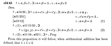
To work our way up, we start even simpler: with a circle. One way to characterize a circle is as a set of points (joined into a continuous line) a fixed, common distance away from a center. Now, how do we single out those points? If we think of a two-dimensional plane, like a sheet of graph paper, we can define every point on it by two numbers—its coordinates, commonly written as (x, y) for the horizontal and vertical coordinate, respectively. Then all we need to know to single out the points on the circle is the good, old Pythagorean theorem: the distance between any two points is given by the length of a straight line joining them, which we can think of as the hypotenuse of a right triangle whose sides are given by the differences in x– and y-coordinates. Thus, every point (x, y) a distance r from the origin (0, 0) fulfills x² + y² = r², or for the unit circle with radius r = 1, x² + y² = 1.

What does this have to do with qubits? Well, as noted, a qubit is the quantum version of an object that can take one of two states, [↑] and [↓] for short. (These are just names, and the brackets [.] are just intended to convey the idea that ‘this is a quantum object’; I could’ve equally well called them [up] and [down] or [0] and [1]. In physics, the so-called Dirac notation is used, which employs a half-angle bracket to signify quantumness, e.g. |↑⟩.) Now, we need to take heed of two peculiarities of quantum mechanics:

1. Any combination of possible states of an object is also a possible state of an object—e.g. with states [↑] and [↓], we also get states of the form a∙[↑] + b∙[↓]
2. The likelihood of finding a system in either of the possible states [↑] and [↓] is given by the square of the corresponding prefactor, i.e. a² and b².

But now we note that since we must find the object in one of the two states, the two options exhaust all possibilities, and thus, their total probability must sum to 1—that is, a² + b² = 1. Consequently, every such state can be represented by a point on the unit circle!

Moreover, since we have made no restrictions on a and b other than that their squares sum to one, they can range from anywhere between -1 and 1—that is, they can become negative. This is a stark difference from classical probability theory, where only positive numbers are admissible—and in a very real sense, it’s the reason for all the quantum weirdness: sometimes, two options that are each admissible on its own differ only by a sign—which then means they cancel each other out. This is quantum interference! This important phenomenon needs a little demonstration.

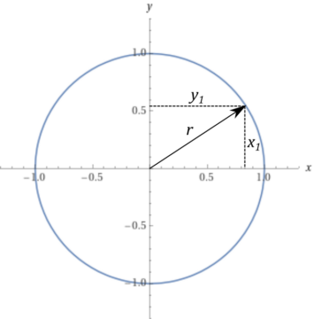
The setup you see here is called an interferometer, and allows for a simple demonstration of quantum interference. Some quantum system—perhaps single photons, or electrons—traverses an obstacle course featuring of (beam-)splitters S and detectors D. The particle can take either the upper path [u] (red) or the lower path [l] (green). The splitters then act as ‘half-mirrors’, letting through or reflecting the particle with 50% probability. Concretely, this means that splitters act on the possible input states as follows:

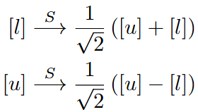
There’s two aspects of this that warrant some further attention. First, the square root of two comes in because probabilities are obtained as the squares of the coefficients, so after the action of the splitter, each possibility is present with probability ½.

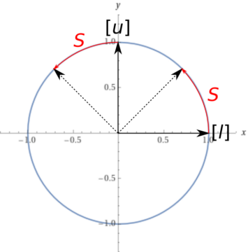
The minus between the two terms in the second row might seem more puzzling. But it has a simple geometric explanation: recall that the valid states for our qubit lie on the unit circle; thus, transformations between states are rotations of the circle (and possibly reflections, but we’ll content ourselves with the rotations for now). If we now somewhat arbitrarily denote the point (0,1) with [l], a rotation of 45° will take that state to the desired combination of [u] and [l] where we will find each with 50% probability. That same rotation, however, will take the state (1,0), standing for [u], to one whose component in [l]-direction is negative.

Now it’s just a simple matter of tracing the states through the transformations effected by the different elements. We start with a particle on the lower path [l]:

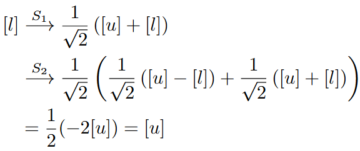
Hence, any particle starting on the lower path will leave the interferometer on the upper path—to be detected by the detector D₁. This might not seem so strange, at first—but recall that we had stipulated that only a single particle traverses the setup at any given time. What does it mean for such a particle to have components traversing the different paths? A classical analysis would have the particle taking either the upper or the lower path at each S; but then, both D₁ and D₂ should detect it half the time.

And indeed: if we insert detectors D₃ and D₄ into the apparatus, each will detect the particle in half the cases; and then, afterwards (provided we have used some non-destructive means of detection), so will D₁ and D₂. This is a discrete analogue of the famous double-slit experiment, with essentially just two possible paths for the particles to take—a phenomenon which, in Feynman’s estimation, contains ‘the only mystery of quantum mechanics’. And all it took was the introduction of a single, innocuous minus sign!

Going 3D

The description above is really just a ‘slice’ of quantum mechanics. The reason for this is that, in the full theory, the coefficients in an expression like a∙[↑] + b∙[↓] are not merely real, but complex numbers. Complex numbers, you might know, are produced from the reals by adding a new element, typically denoted simply i and defined as the square root of -1. This might seem somewhat strange, at first: negative numbers don’t have square roots! But here, again, thinking about rotations in the plane can help.

We start out with a rigid rod of length 1. Then, we can think about the positive real numbers as dilations: the number 2 doubles it in length, ½ halves it, π makes it roughly 3.14 times as long. Negative numbers are also readily explained: they just flip the rod through the 0-point, and then stretch it. So -3 turns it over by 180°, then triples its length, and so on. But once we start flipping, why stop there? Why not, say, rotate the rod by 90°?

But what number would this operation correspond to? Well, we know that rotating twice by 90° gives a rotation by 180°. And compounding our operations is just done by multiplication: stretching by a factor of two, then flipping and stretching by a factor of three, is equal to flipping and stretching by a factor of six. So whatever number this rotation corresponds to, this means that multiplying it by itself must equal -1—and there we have it: it’s just i, the square root of -1. Nothing strange about that at all!

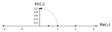
The imaginary unit i rotates the number line into a plane, and every point on that plane yields a complex number, which we can decompose into a ‘real’ and an ‘imaginary’ part—despite the names, not really anything more ‘complex’ than the x and y coordinates we used earlier. Now, what does this do to our qubits?

If a and b in a∙[↑] + b∙[↓] now are complex numbers, that means we must understand how these coefficients are now related to the probabilities of finding each of the possible states. Luckily, though, there’s a simple way to square a complex number: if a_r and a_i are the real and imaginary ‘coordinates’ of the number a, respectively, then we have just that a² = a_r² + a_i²—that is, we just sum the squares of the two components. But now recall that we need a total sum of 1—thus, from our earlier a² + b² = 1, we now get a_r² + a_i² + b_r² + b_i² = 1, four components instead of two. This is now no longer a simple circle in the plane, but characterizes a set of points at a distance of 1 from the origin in a four-dimensional space! This is the sphere in four dimensions, S³. (Why three instead of four? Just as, in two dimensions, the ‘two-dimensional sphere’, or the circle, is a one-dimensional object (a line), the boundary of a disk centered on the origin, S³ is the three-dimensional boundary/surface of a four-dimensional ‘ball’ of radius 1.)

This is a little hard to visualize! But there is a property of quantum mechanics that we can use to ‘slim down’ our representation a bit: overall rotations of the state don’t matter. Recall that only the probabilities given by a² respectively b² have physical significance. If I multiply both of these with the same complex number of length 1—i.e. I perform a ‘pure’ rotation without stretching anything—then these won’t change (just as a² and (-a)² are the same). But that means I can always rotate my state such that, say, a is a real number—leaving me with only three ‘free’ parameters for the state (which I’m just going to go ahead and call x, y, and z). These then again fulfill x² + y² + z² = 1—the equation for a sphere in three dimensions (S²). Consequently, each state of a single qubit can be represented by a point on the surface of a three-dimensional sphere—the so-called Bloch sphere.

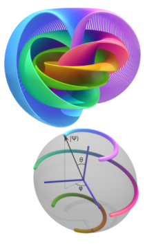
But now the circle closes: the construction described above is just a different way of looking at the Hopf fibration, the topic of the previous column. The four-dimensional sphere S³ is decomposed into the three-dimensional Bloch sphere (S²) and an S¹-fiber associated to each point.

This is a picture that will take some getting used to, but ultimately, yields a simple and intuitive image of a single qubit. All that such an entity is can be represented by a point on a three-dimensional sphere; and all that we can do with it is given by rotations on that sphere.