
by David Kordahl
The science lab and the theory suite
If you spend any time doing science, you might notice that some things change when you close the door to the lab and walk into the theory suite.
In the laboratory, surprising things happen, no doubt about it. Depending on the type of lab you’re working in, you might see liquid nitrogen boiling out from a container, solutions changing color only near their surfaces, or microorganisms unexpectedly mutating. But once roughly the same thing happens a few times in a row, the conventional scientific attitude is to suppose that you can make sense of these observations. Sure, you can still expect a few outliers that don’t follow the usual trends, but there’s nothing in the laboratory that forces one to take any strong metaphysical positions. The surprises, instead, are of the sort that might lead someone to ask, Can I see that again? What conditions would allow this surprise to reoccur?
Of course, the ideas discussed back in the theory suite are, in some indirect way, just codified responses to old observational surprises. But scientists—at least, young scientists—rarely think in such pragmatic terms. Most young scientists are cradle realists, and start out with the impression that there is quite a cozy relationship between the entities they invoke in the theory suite and the observations they make back in the lab. This can be quite confusing, since connecting theory to observation is rarely so straightforward as simply calculating from first principles.
The types of experiments I’ve had been able to observe most closely involve electron microscopes. For many cases where electron microscopes are involved, workers will use quantum models to describe the observations. I’ve written about quantum models a few times before, but I haven’t discussed much about how quantum physics models differ from their classical physics counterparts. Last summer, I worked out a simple, concrete example in detail, and this column will discuss the upshot of that, leaving out the details. If you’ve ever wondered, how exactly do quantum models work?—or even if you haven’t wondered, but are wondering now that I mention it—well, read on.
A complicated instrument, briefly described
Most readers, at one time or another, have probably had a chance to use a light microscope. Just like in everyday life, light shines on an object, and bounces off. By using lenses to bend this light, one is able to observe much smaller structures than would be visible otherwise. Physics purists will note that there is something already quantum about light microscopes, since everyday light can be described using photons. But the quantum character of basic observations becomes much more obvious in electron microscopes, for which classical models are just used as a stepping-stone to quantum interpretations, and we now turn our attention toward these cantankerous wonders.
Electron microscopes are typically larger and more fiddly than light microscopes. Light travels largely unimpeded through air, but for electrons to make it from the electron gun to the electron detector, the body of the electron microscope must have the air pumped out. Furthermore, light can be focused using glass lenses, but the “lenses” in an electron microscope are just electromagnets that can be “focused” by adjusting their currents.
I’m going to describe one type of quantum observation that can be done with an electron microscope, which has the professional name of electron energy-loss spectroscopy (EELS). To help visualize this, take a look at Figure 1 below, which I have stolen from the website of Gatan, Inc., an electron microscope manufacturer. There are quite a few details in this cartoon, but it will be best to focus on just three things: the electron source (top), the TEM sample (down a bit), and the EELS system (bottom).
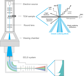
This is a “TEM,” which stands for transmission electron microscope. The “transmission” part means that the “sample,” the thing you’re shooting electrons at, is typically thin enough for the electrons to breeze right through. The basic story is that electrons are sprayed down by the electron gun, interact with the sample, and are then collected at the bottom. In EELS, what is measured is how much energy the electron loses in its travel from top to bottom (hence “electron energy-loss spectroscopy”). For such measurements to be informative, the energy of each electron has to be monitored at both the beginning and end of its flight. So does the initial energy of the sample. I won’t get into it here—too hard—but this involves more electromagnets and liquid nitrogen.
How much of this mess makes it into the theory suite? Not much. The “spectroscopy” part of EELS means that we want to keep track of how much energy the electrons will lose as they interact with the sample, and with what probability. These are the basic quantities that our model will predict.
A simple model with “off-the-shelf” parts
Models for real samples typically include quite a bit of physical detail, linking various measurable qualities together in ingenious ways, but there are circumstances where simple models will do the trick. Every physicist’s favorite go-to model is the harmonic oscillator—basically, a spring-tethered particle that, once it starts going back and forth, continues to oscillate forever. This abstraction that can be used to describe all sorts of underlying phenomena, from swaying bridges to quantum fields, but let’s think now of something like a little molecule that get stretched out as an electron whizzes past it.
Let’s describe the TEM sample as a harmonic oscillator, and electron as a free particle. The reason to play with basic models like the harmonic oscillator and the free particle is that these can be picked up “off the shelf,” as it were. Since the ins and outs of these models are thoroughly understood, any novelty here will be relegated to the interactions between the parts.
I’ve tried to illustrate such an interaction in Figure 2 below. To keep the model simple, our electron just moves along one direction, and we track its position with the variable x. We pin the oscillator to some fixed position, such that the closest the electron will get to the oscillator is some distance b when the electron is at x=0. As far as the oscillator goes, we track the its displacement with the variable y. Finally, we propose some initial conditions—an initial speed of v0 for the electron when it is far away from x=0, say, and an oscillator that’s initially motionless, with y=0.
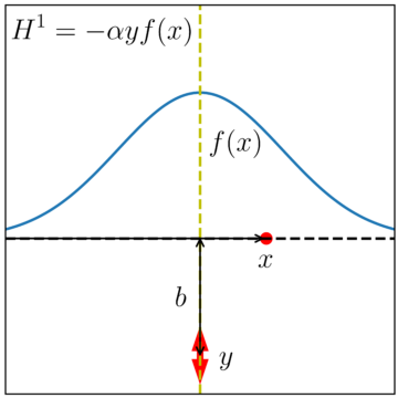
If the electron and the oscillator never interact, their behavior will be very simple, with the electron simply zipping along without slowing down, and the oscillator—our stand-in for the TEM sample—never absorbing any of the electron’s energy. Anything interesting that goes on will happen because of the potential energy that arises when the oscillator and the electron interact. The form I’ve chosen for this potential energy is the product a function “f(x)” that’s large when the electron is close to the sample and small when the electron is far away; “y,” the displacement of the oscillator; and “ɑ,” a constant that fixes how strong the interaction is and gives the overall product sensible units.
With this in place, we’re ready to make predictions. Let’s go.
Kicking a classical oscillator
So how, exactly, can we make these predictions? If we stay in the realm of classical physics, the answer is simple. If we know what all parts of the system are doing at one instant in time—or, more carefully, if we know the positions and velocities of each of our point particles at some initial time—then we can just use Newton’s laws of motion to predict the positions and velocities of each of these point particles at any later time.
So what happens for the model with a coupled electron and oscillator? For the initial condition we have discussed (fast electron starts out far away from motionless oscillator), the outcome is also simple. As the electron passes by, it loses a little energy—i.e., it slows down. The system’s total energy stays constant, so this loss of energy by the electron requires an energy gain by the sample, so the oscillator now oscillates.
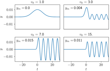
The amount of energy that is deposited into the oscillator by the electron depends on the initial speed of the electron. I’ve plotted a few examples below in Figure 3. In these plots, v0 is the initial speed of the electron, and ym is the final amplitude of the oscillator, whose final motion bobs from –ym is to +ym. For electrons that start out too slow or too fast, little energy is transferred. For this example, the most energy is transferred from the electron to the oscillator when the electron’s initial speed is tuned to v0 = 7.
So what’s wrong with this? Why shouldn’t we go about developing this sort of model, with different interactions for different circumstances?
The primary reason is that, at least according to the usual way of thinking about things, this doesn’t model what actually happens. Remember the experiment we’re trying to model. Experimenters do their very best—using the liquid nitrogen and fancy electromagnets—to make sure that the electron and the sample have the same initial conditions each time around. But our classical model has the electron lose the same amount of energy every time it interacts with the sample, and this isn’t what happens.
What happens is that sometimes the electron loses energy, but often it will pass by the sample without losing any energy. This means that we’re in the realm of probabilities and should build models that accommodate this.
Entanglement and wavefunction branching
Okay, so what changes when we treat this as a quantum model? Where do the probabilities come from? Do we roll virtual dice or something?
Surprisingly, no. The setup is very similar to that of a classical system. As before, we set up our system with some initial conditions. Just as before, the initial conditions predict the state of the system at any later time. But beyond these similarities, there are real differences in the quantum story.
First of all, the free particle—our electron—is replaced by a quantum free particle, and the harmonic oscillator—our TEM sample—is replaced by a quantum harmonic oscillator. How does this differ from what we’ve already done? One notable change is that each of these objects is now smeared out, such that the initial conditions of our system aren’t just a list of four numbers (x, vx, y, vy), as in the classical case, but instead is formed from the product of two complex functions—e.g., like ψ(x)ψ(y).
Second, instead of Newton’s laws predicting how the state of the system evolves in time, we will use the Schrodinger equation. Still, the way the system changes in time is just a deterministic math rule, so this isn’t much of a difference, at least not until measurements come into the picture.
Let’s start slowly. Suppose we just replace our oscillator with a quantum oscillator, but keep our old classical electron. How would that be different?
Well, the outcome wouldn’t really too different from the classical outcome. As you can see in Figure 4, the quantum harmonic oscillator in its lowest possible state looks a lot like a smeared-out wave, and when it is kicked by a classical electron, its probability density wobbles back and forth. The magenta line shows the average position of the quantum oscillator, which exactly matches the classical outcome of Figure 3 above.
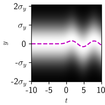
But this similarity doesn’t completely capture the novelty of what happens when the full wavefunction evolves. For that, we need to smear out the electron, too.
As everyone has heard by now, quantum particles follow Heisenberg’s uncertainty principle, so if we fix the electron’s momentum px, this will increase the spread of the electron’s position x. For the purposes of energy-loss spectroscopy, it will be more important to know about the electron’s momentum—and hence its energy—than about its position. This means the wavefunction ψ(x) for the electron will start out with nonzero values over a large range of x, to accommodate a sharp initial momentum p0.
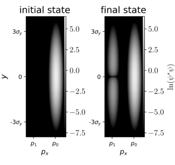
In Figure 5, I have tried to illustrate this joint wavefunction in px and y, that is, for the electron momentum and the oscillator position. On the left, we see the “initial state” wavefunction from before the electron and the oscillator interact. On the right, we see the “final state” wavefunction from after the electron and the oscillator have finished their interaction. Because we can’t write the final state as a simple product ψ(px)ψ(y) anymore, we say that this final state is entangled. The final state wavefunction has nonzero values for two distinct electron momenta, representing two possible outcomes.
The final state wavefunction, here, looks like it has two “branches,” one where the electron ends up with a slightly decreased momentum p1, and another where the electron keeps its initial momentum p0. These outcomes represent, respectively, one case where the electron and the oscillator have exchanged energy, and one case where they haven’t.
Finally, we need to link the wavefunction to experimental predictions. The probability of landing in each branch just depends on the relative proportion of much of the wavefunction density |ψ(px,y)|2 is present in each branch. With this interpretation, we now have, as promised, a model that predicts how much energy the electrons can lose during their interactions with the sample, and with what probability. Hooray!
But…wait a minute. Is that it? Are we done?
Theories and the world
Let’s return, for a moment, to our initial worries about the science lab and the theory suite. Just about everyone agrees that quantum models help us predict the correlations and probabilities observed in delicate experiments involving microscopic objects. But people disagree sharply about what these models mean. At one extreme is the dismissive position that the wavefunction is just a mathematical abstraction we use to make predictions, having no further metaphysical importance. At the other extreme is the position that the universal wavefunction is actually all there is, and that the goal of our study should be to understand where we exist within that higher reality.
My own feeling is that it’s a good thing to take our theories seriously, to acknowledge that features like quantum entanglement and wavefunction branching are natural features of quantum theory, while, at the same time, holding in mind the fact that the world itself is distinct from any quantum model of it. It’s fun to hang out in the theory suite, but only in the science lab can we experience the real thing.