
by Jonathan Kujawa

Some years ago we discussed Brobdingnagian numbers. You can find the 3QD essay here. These are numbers that are so mind-bogglingly large they defy human imagination. Perhaps the most famous is Graham’s number. It’s so large I can’t write it down for you. It’s not that I refuse to write it down; I can’t. If I used one Planck volume per digit, Graham’s number would take up more than the observable universe [1]. Still, we would like to use and study such numbers and other hard-to-contemplate mathematical objects.
With the advent of computers and computer science, one reasonable way to describe a mathematical object is via a computer algorithm. That is, a step-by-step recipe that describes the number or question we are interested in and that could (at least in principle) be implemented on a computer. This is a pretty reasonable way to ringfence the parts of mathematics on which we might claim our minds can handle (maybe with help from computers).
For example, computable numbers are real numbers that are knowable in this sense. If we want to know the number’s nth digit, we can write down an algorithm that computes that nth digit for us. Even though the digits of π go on forever and have no discernable pattern, we have such algorithms for the digits of π, so it is computable. Likewise, there is a recursive formula for Graham’s number. It, too, is computable.
We aren’t limited to numbers. In a pair of 3QD essays last year (here and here), we saw that mathematicians have made significant progress in turning mathematics and mathematical thinking into things a computer can work with. There we saw machine learning help mathematicians make new connections and insights, and theorem verification software can help check the validity of results.
Before getting too cocky, it is worth remembering that we learned that most real numbers aren’t computable. Things that are computable go far beyond our everyday experience, but we shouldn’t forget there are vast seas beyond computable’s shores.
With this in mind, it is perhaps worth trying to understand the limits of what is computable.
To do this means we need to agree on a good working definition of “computable”. Most folks agree that a good starting point is the Turing machine. We talked about them a bit here at 3QD.
In Turing’s original paper, the machine had an alphabet of symbols it could read and write, an infinite strip of paper to read from and write on, and a list of rules. In one run of the machine, it will read what is written at the current location on the paper strip, look up the rule corresponding to that symbol and perform whatever action(s) the rule demands. The actions might include replacing the symbol in the paper strip with a possibly different symbol as well as moving the head left or right to a new location on the strip. By choosing the alphabet and the rules, you can “program” the machine. You start it at some location on the strip and let it run in a loop over and over until it stops. If you’ve programmed it correctly, when the machine halts it will have added two numbers, computed a digit of π, rendered a Pixar movie, checked your proof of the Riemann Hypothesis, or done whatever else you might have asked it to do.
The main idea is that any step-by-step algorithm (and, hence, any software) can be encoded into a Turing machine. If you’d like your own pocket computer, you can print a business-card-sized one from the website of Alvy Ray Smith. Importantly, just like your computer, a badly programmed Turing machine might never stop running. If it doesn’t halt, it never completes the task we set.
In short, understanding what is computable boils down to understanding what can be encoded in a Turing machine which eventually halts.
 This brings us to the Busy Beaver function. It is a measure of how long a Turing machine might run before it halts. Indirectly, the Busy Beaver function tells us something about how complicated things can be while still being computable. It was first introduced by Tibor Radó in 1962 and is actively studied to this day. Indeed, we have many more questions than answers about the Busy Beaver. I first learned about the Busy Beaver from an interesting survey article by Scott Aaronson. You can find the survey article, plus further discussion and links on his blog. In particular, you’ll find an interesting discussion by various researchers and hobbyists about open problems and conjectures involving the Busy Beaver function and variants.
We’ll follow Aaronson and Radó by talking about a modified and simplified version of Turing’s original machine [2]. We have a Turing machine with the following features:
- The symbols are 0 and 1.
- We have a long strip of paper that can be read, written on, and erased.
- We have a read/write/eraser head that can travel back and forth along the paper strip.
- A list of “states”. At any moment, the machine is in one of these states.
- A list of rules. For each state, there is a rule for 0 and a rule for 1. Each of the rules will tell the machine to write a 0 or 1 in the present location on the strip, possibly change itself to a new state, and to move one step left or right on the paper strip. Alternatively, the rule can tell the machine to Halt.
In each run of the machine, it reads a 0 or 1 from the paper strip and then, based on the machine’s state, executes the rule corresponding to the 0 or 1 it read. The machine is put into a start state and placed on a strip of paper filled with all zeros. As before, you let the Turing machine run over and over until it halts.
Here is a schematic of a Turing machine with two states (state A and state B). It is placed on the tape and is started in state A, and ends up running six times:
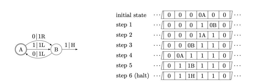
In step 1, the machine is in state A. It reads a 0. According to the schematic diagram, this means it should replace the 0 with a 1, move one step to the right, and change its state to state B. At the next step, since it reads a 0 and now is in state B, the rule says to replace the 0 with a 1, go one step to the left, and change its state to state A. The machine will keep running until it reads a 1 while in state B. That is the only time it halts.
Radó asked a seemingly simple question. If you tell me how many states you will use (say 2, like in the example), there are only finitely many possible rules and so only finitely many possible Turing machines. Let’s throw away the ones which never halt. The ones which remain stop after some number of steps. If we want to understand how bad/complicated something can be while still being computable, then we’re interested in the worst case: how long can a Turing machine with n states run and still halt?
That is, if you are considering n states, we define the Busy Beaver number BB(n) to be the number of steps taken by the Turing machine that ran the longest before halting. There are only finitely many Turing machines with n states which halt. In principle, you can run them all, count the number of steps each takes until it halts, and figure out which took the longest. Easier said than done! When n=2 states, there are 6,561 possible Turing machines.
We know that BB(2)=6. That is, the longest run of a Turing machine with 2 states is 6 steps. This is the machine given in the example. We also know BB(3) and BB(4). If your Turing machine has 5 states or more, we have little to no idea how long it could run before halting! Here’s the current state of the art:
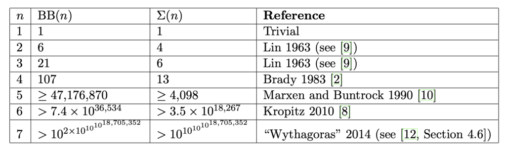
This table gives lower bounds on BB(n) (and for the related quantity Σ(n)) along with references. Look at the row for n=5. Something amazing is true for Turing machines with 5 states. There are only 25 such Turing machines that remain to be analyzed. The current record is one that takes 47,176,870 steps to halt. By running the remaining 25 on a computer, we know they all run for at least 100 billion steps. If none of them halt, BB(5) = 47,176,870. If one of them halts, then it’s the new champ, and BB(6) is at least 100,000,000,000.
For reference, there have been about 9 x 1060 Planck seconds since the Big Bang. From the table, we see BB(6) is vastly, hugely, staggeringly larger. There is a Turing machine with just 6 states that could have been running furiously since the beginning of our universe and would hardly have gotten started.
Of course, BB(7) is ridiculously large, and BB(8), BB(9), etc., are even more so. For example, B(18) is known to be larger than Graham’s number! It’s hard to even conceive of, say, BB(1,000,000). It is an open area of research to obtain better bounds on BB(n) [3].
The Riemann hypothesis is the most famous open problem in mathematics. Matiyasevich, O’Rear, and Aaronson showed that there is an explicit 744-state Turing machine that halts if and only if the Riemann hypothesis is true. Of course, BB(744) is so large that it is quite likely that this Turing machine will run without halting right up until the heat death of the universe.
There are also connections between the Busy Beaver and the very foundations of mathematics. Whether or not the set-theoretic and logical foundations of mathematics are sound can be verified by explicit Turing machines halting (or not). If you could find a shortcut to figuring out if a Turing function halts or not, you could answer all these deep questions. The safer bet is there is no such shortcut!

[1] A Planck volume is so small that there are more Planck volumes inside a cubic meter than there are cubic meters in the known universe.
[2] If you use n states, there is a total of (4n+1)2n possible Turing machines. So in the example, when n=2, there are 6,561 possible Turing machines. The one given above is just one of them.
[3] Warning! If you want to try to find an upper bound on how big BB(n) can be, you should know that it has been proven that if f(n) is any computable function, then BB(n) is bigger than f(n) for n sufficiently large. So any limits on BB(n) are necessarily uncomputable!