
by Jonathan Kujawa
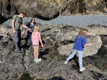
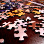
My nieces, Hannah and Sydney, came to visit for the weekend. Since they’re 8 and 9, the delightful Guardian Games in downtown Corvallis was a must-stop. Along with games galore, they have an amazing assortment of puzzles. They have puzzles with micro-sized pieces, puzzles with jumbo-sized pieces, puzzles with only a few pieces, and puzzles with a veritable googolplex of pieces.
The profusion of puzzles reminded me of a recent research paper in applied geometry. The authors are Madeleine Bonsma-Fisher, a mathematician and data scientist at the University of Toronto, and her partner Kent Bonsma-Fisher, a quantum computing and optics researcher.
 Like many of us, they assembled an inordinate number of puzzles during the COVID-19 restrictions. And like many puzzlers, they came to wonder:
How big a table do you really need if you want to assemble a puzzle?
Everyone knows you need extra room on the table to spread out the pieces. But how much extra room? Does the amount of space needed depend on the size of the pieces? Or if the puzzle has more or fewer pieces?
This is a frequent topic of discussion for puzzlers on the internet. A commonly cited rule of thumb is that the table should be twice the area of the finished puzzle.
But rules of thumb aren’t math. Fortunately, close readers of 3QD know of some math that could help here. We discussed the problem of sphere packing here and here. Sphere packing is all about finding an arrangement of equal-sized spheres (e.g., cannonballs or oranges) that packs the most spheres into a given volume.
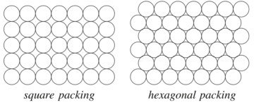
Cannonballs and oranges live in three dimensions, but you can ask about packing spheres in higher dimensions like we did in those essays. But you can also ask the question in two dimensions. There it becomes a problem of packing equal-sized circles on a tabletop. And if you’re a mathematician, a circle is basically the same thing as a puzzle piece!
In 1892 Thule [1] proved that a hexagonal packing of circles is the densest configuration. Even my nieces can quickly figure out that the rectangular packing is pretty good, a hexagonal packing is better, and it is hard to imagine anything could beat it. But proof by lack of imagination isn’t good enough. When Kepler first thought about sphere packing in 1611, he no doubt already knew that hexagonal packing was as good as it gets, but it took 250+ years for us to know for sure.
 The Drs. Bonsma-Fischer said: Well, if you have a puzzle with area A with N pieces of roughly the same size, then each piece should have area A/N. Since we’re mathematicians, we can assume each puzzle piece is a square and has side length √(A/N). But when the pieces are flat on the table, they could be turned any which way, so each one actually needs the room of a circle just big enough to contain that square [3]. If you do the geometry, you discover that the circle has diameter d=√(2A/N).
So we’ve reduced ourselves to packing circles of that size on a tabletop. The best packing method will use the least space on a table, so the best we can do is the hexagonal packing. Using observation, we can calculate how much area the unassembled puzzle needs. Amazingly, the number of pieces and their size washes out in the calculation! When you do the calculation, you get:
Area of unassembled puzzle = √3 x Area of Assembled Puzzle.
But √3 ~ 1.73. When all is said and done, the calculation says an unassembled puzzle takes about 1.75 times the area of the assembled puzzle. See their paper for the details of the computation.
You might be skeptical. After all, we made a lot of simplifying assumptions. Maybe in the real world, the number or size of pieces is important. Drs. Bonsma-Fischer and their son also collected real-world data. They:
completed 9 different puzzles of varying sizes and numbers of pieces and measured their unassembled and assembled areas. Before assembly, we laid out all the pieces in a flat layer in an approximate circular shape. We attempted to make this process realistic to real-world puzzle solving by not being too precise about getting the pieces as close together as possible.
They measured the area of the disassembled and assembled puzzles and plotted the data along with a dashed line marking the theoretical result:

This is one of those rare cases where the data matches the model, and where both match the practitioner’s rule of thumb. A triumph of theory, laboratory data, and real-world application!
Let me mention that the entire discussion in this essay assumes that the puzzle pieces are nearly equal in size. It becomes a much harder problem if some pieces are bigger than others. Here, even the two-dimensional problem is mostly unsolved. Packomania summarizes some of what is known.
[1] Actually, the history is a little complicated. Evidently, in 1773, Lagrange proved the hexagonal configuration was the densest among the “lattice” configurations (the regular, repeating ones), and in 1892, Thule showed that it was still the densest even if you allow irregular configurations. However, Thule’s argument was generally judged to be incomplete, and it wasn’t until 1942 that Tóth gave a completely rigorous proof of Thule’s claim. It goes to show you that what is true in math depends on what you are allowed to assume and what you count as a complete proof. Math is very much a human endeavor.
[2] Image from Wolfram Mathworld.
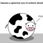
[3] Insert your favorite Spherical Cow joke here. The image is from Abstruse Goose. Their webpage seems to be offline, sadly!