
by Jonathan Kujawa

The most fundamental example of a function is a polynomial. Everyone sees polynomials in school. These are the functions whose rules involve taking the input to powers, perhaps multiplying by numbers, and perhaps doing some additions and subtractions. For example,
![]()
Here the input variable is x. When you input x= 2 or x=1 or x=-1, you get p(2)=3, p(1)=2, and p(-1)=6 as outputs.
You may recall that a zero (or root) of a polynomial is the name for an input that happens to give you zero as an output. For example, the polynomial x² – 4x + 3 has zeros x=1 and x=3. On the other hand, the polynomial p(x) doesn’t seem to have any zeros.
Many applications in and out of math come down to the question of finding the zeros of a polynomial. Several years ago, we talked here at 3QD about how certain geometric constructions from Ancient Greece are impossible with ruler and compass, but become possible using origami. Under the hood, this came down to understanding the zeros of certain polynomials. Important parts of number theory and geometry are essentially about the problem of understanding the zeros of polynomials.
I was recently reminded that even simple polynomials can have beautiful and remarkable zeros. A Littlewood polynomial is a polynomial where the numbers in front of the powers of x are only allowed to be 1 or -1. Here are a few examples of Littlewood polynomials:
Notice that there are no numbers in the rules of these polynomials except for 1 and -1. Littlewood was a famous British number theorist from the first half of the twentieth century. He seems to be one of the first to study the zeros of these polynomials.
Before we continue, I should make clear that Littlewood considered the complex number as fair game when looking for zeros. If you use the quadratic formula on p(x) from above, you’ll find that it has roots x = 1 – √-2 and x=1+√-2. In school, we are taught that taking the square root of a negative is forbidden. This is nonsense! If you forge ahead, nothing bad happens. Indeed, you find that you’ve just invented the complex numbers. They have the delightful property that they contain every root of every polynomial. They are where you want to be if you are thinking about the roots of polynomials [1].
One perk of using the complex numbers is that each complex number can be written in the form a+b√-1, where a and b are real numbers. When you have a pair of real numbers, you should immediately think to plot the point (a,b) on the xy-plane. You’ve just turned numbers and algebra into geometry!
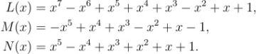
So what happens if we write down a few hundred thousand Littlewood polynomials, find their roots, and plot those roots on the xy-plane? In 2006 Dan Christensen and Sam Derbyshire did just this. They plotted the roots for every Littlewood polynomial whose biggest power of x was 24 or less. Something surprising and beautiful emerges:
If you want to magnify the image to see the details, this link gives you a zoomable version. Each illuminated pixel is the root of a Littlewood polynomial. We immediately notice the bright areas where roots cluster together, and the near-black areas where they seem to be very sparse.
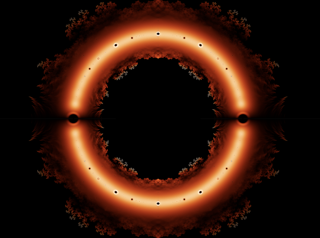
For example, there is a little black disk on the east side of the picture that is centered at x=1. Certainly, x=1 is the root of a Littlewood polynomial (for example, x – 1). But it also appears that x=1 “repels” other zeros from its neighborhood. Zooming in, we see the following picture.
If you look closely, you’ll see a complicated pattern along the rim of the dark disk. You might also notice the thin line across the equator of the black disk. That’s not a glitch; it is a line of zeros that are real numbers. For some strange reason, x=1 repels the complex zeros, but not the real zeros. But if you look even closer, you’ll see that even the real roots can’t get too close: there is a gap in the line at the center of the disk.
We also notice that there is a symmetry to the big image. While the clustering and repelling behavior is mysterious, the symmetry can be explained. It is not too hard to see that if z is a root, then so is -z, 1/z, and the complex conjugate of z [2].
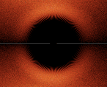
Looking more closely, we see fractal-like fringe along the inside and outside edges of the big bright circle. Greg Egan wrote a web app that lets you dynamically zoom in. I picked a more-or-less random spot in the northwest corner along the inside rim. Here’s what you see:
In case you wonder, Greg Egan chose a different scheme for coloring the pixels in order to highlight other aspects of the image.
Mathematicians have been able to prove some things about the behavior of these zeros. Even as you let the power of x get bigger and bigger, the zeros of the Littlewood polynomials all lie in the donut-shaped region shown in the above image. None get too close nor too far from the center [3]. On the other hand, Thierry Bousch proved in 1988 that, as the powers of x increase, the image fills in with ever more pixels. That mysterious hole caused by x=1 repelling its neighbors eventually fills in almost completely [4]. We know how to explain some of the features that appear when you study the distribution of zeros of polynomials, but there is just as much we don’t know.
It turns out that the Littlewood polynomials aren’t the only polynomials with beautiful roots. It has been known for a while that if you limit yourself to a small set of possible numbers in front of the powers of x, this frequently causes fractal-like behavior. Odlyzko and Poonen studied the case when you only allow 1 and 0 as the numbers. Folks have created web apps that let you play with various families of polynomials to see what their zeros look like when plotted.
Another rich source of polynomials are the characteristic polynomials of interesting matrices. These polynomials are used all the time in Linear Algebra. Undergraduates love to hate having to compute them. What sent me down this rabbit hole in the first place was a recent post by Dan Piponi on Mastodon. He plotted the roots of the characteristic polynomials of a bunch of matrices and showed they exhibit a similar fractally behavior:

If we go into the weeds for a minute, we’ll see that this is maybe not entirely unexpected. A matrix is an array of numbers. Dan Piponi started with a matrix where if you looked at any individual row or column, you would see all zeros except a single entry, and that single entry would be a 1 or a -1. He then added two of those matrices together by adding the matching entries. The result would be a matrix with almost all zeros, a lesser number of 1’s and -1’s, and rarely a 2 or -2 (if the two matrices happened to have 1’s or -1’s in matching positions).
The characteristic polynomial is calculated using the matrix entries, so the numbers in the polynomial will be constrained by the fact we start with 0’s, 1’s, -1’s, and the occasional 2 or -2. Experience shows that the zeros tend to have unusual, fractal-like behavior when you severely limit the possibilities for your polynomials.
Still, as far as I know, it is a complete mystery what’s going on in this plot. Is it like the Littlewood polynomials where the gaps eventually fill in? Are there limits to where the zeros can be? We can already see from Dan Piponi’s plot that there isn’t a big hole in the center like there was for the Littlewood polynomials.
Once again, math hints at worlds waiting to be discovered!
[0] Image borrowed from here.
[1] It turns out they are also where you want to be if you are doing modern physics. Quantum physics and quantum computing fundamentally depend on the complex numbers. Not only are the complex numbers not complex, they are just as real as the real numbers!
[2] If z = a + bi is our complex number, then its complex conjugate is the number a – bi.
[3] Specifically, the zeros are all at least 1/2 a unit from the center, but not more than 2 units from the center.
[4] If you are only interested in zeros that are real numbers, then the conjecture is that every real number in the region [-2, 1/2] and [1/2,2] is a root of some Littlewood polynomial. See this interesting student thesis for some evidence in favor of the conjecture.